Chebyshev Interpolation: an interactive tour
Scott A. Sarra
Marshall University
1 Introduction
Most areas of numerical analysis, as well as many other areas of
Mathematics as a whole, make use of the Chebyshev polynomials. In
several areas, e.g. polynomial approximation, numerical
integration, and pseudospectral methods for partial differential
equations, the Chebyshev polynomials take take a significant role.
In fact, the following quote has been attributed to a number of
distinguished mathematicians:
"The Chebyshev polynomials are everywhere dense in numerical
analysis."
In this manuscript we make use of Java applets to interactively
explore some of the classical results on approximation using
Chebyshev polynomials. We also discuss an active research area that
uses the Chebyshev polynomials. References
[14,15] are devoted to the Chebyshev
polynomials may be consulted for more detailed information than we
provide in this brief presentation.
2 Overview of the Applets
The applets used are the:
- Chebyshev polynomial (CP) applet.
- The CP applet plots
the degree zero to degree twelve Chebyshev polynomial. The
degree of the polynomial can be changed by changing the value
of the slider at the bottom of the applet.
- Chebyshev approximation (CA) applet.
- The applet visualizes
the interpolatory, the continuous, the discrete, and the filtered
Chebyshev approximations of several functions. The functions are described in section
8 below. The functions can be selected in
the applet from the Functions menu at the top of the
applet. The applet contains two windows. In the left window
the exact function is plotted in black. Up to two
approximations can be plotted (the first in blue and the second in red)
and compared by making selections from the Approximations
menu. By default the approximation error is displayed in the
right window. The magnitude of the Chebyshev coefficients can be displayed in
the right window by selecting plot coefficients from the Options
menu. The y-axis of the error or coefficient plot can be displayed on a log scale by
selecting semiLogY from the Options menu. The plot CGL
points option marks the exact value of the interpolated
function in the left window with a green dot at the
interpolation sites. The connect (right) option on the
options menu, when left unchecked, allows the error plot to be
displayed without the points on the graph being connected.
This sometimes produces a more pleasing plot on a semilog
scale when values are near zero. A parameters dialog can be displayed by pressing the parameter
dialog option from the options menu. From the dialog the order of the exponential filter may be
changed as well as the number of evenly spaced points NP at which the
interpolants are evaluated.
- Runge phenomenon (RP) applet.
- The RP applet illustrates the
divergence of equidistant polynomial interpolation by using a
classic example.
- Exponential filter (EF) applet.
- The EF applet plots the value of the
exponential filter of degrees 2 to 32 by changing the value
of the slider at the bottom of the applet. The value of
the filter is plotted versus the normalized coefficient number
n/N. The applet visualizes how much each Chebyshev coefficient is
modified by the filter.
3 Chebyshev Polynomials
The Chebyshev Polynomials (of the first kind) are defined
as
|
Tn(x) = cos[ n arccos(x) ]. |
| (1) |
They are orthogonal with respect to the weight w(x) = (1-x2)-1/2 on the interval [-1,1]. Intervals [a,b] other
than [-1,1] are easily handled by the change of variable x� [1/2][ (b-a)x + a + b ]. Although
not immediately evident from definition (1), each
Tn(x) is a polynomial of degree n. From definition
(1) we have that T0( x ) = cos(0 ) = 1
and T1( x ) = cos(arccosx) = x. For n � 1 we have
the triple recursion relation
|
Tn+1(x) = 2 x Tn(x) - Tn-1(x) |
| (2) |
which can be shown to be true using basic trig identities. Using
equation (2) we see
| |
|
| |
| |
|
|
2x (2x2 - 1) - x = 4x3 - 3x |
| |
| |
|
|
2x (4x3 - 3x) - (2x2 - 1) = 8x4 - 8x2 + 1 |
| |
| |
|
| |
|
and that the Chebyshev polynomials are indeed polynomials of
degree n.
Applet Activity.
What do the Chebyshev polynomials look like? The Chebyshev
polynomials of degree k=0,1,�,12 can be plotted in the CP
applet below. Notice that |Tn(x)| � 1. Since Tn(x) is a
degree n polynomial we can observe as expected that it has n
zeros, which in this case are real and distinct and located in
[-1,1].
Exercise.[Zeros of the Chebyshev polynomials.]
Show that the zeros of Tn(x) are
|
xk = cos |
�
�
|
p(2k+1)
2n+2
|
�
�
|
, k = 0,1,�,n |
| (3) |
The zeros are known as the Chebyshev-Gauss (CG) points.
4 Continuous Chebyshev Expansion
The infinite continuous Chebyshev series expansion is
where
|
an = |
2
p
|
|
�
�
|
1
-1
|
(1-x2)-1/2 f(x) Tn(x) dx. |
| (5) |
Truncating the series after N+1 terms, we get the
truncated continuous Chebyshev expansion
|
SN (x)= |
N
�
n=0
|
�an Tn(x). |
| (6) |
The single prime notation in the summation indicates that the
first term is halved. There are several functions in which the
integral for the coefficients an can be evaluated
explicitly, but this is not possible in general. Examples included
in the CA applet for which a continuous truncated expansion can be
derived are the sign function (32),
f4(x)=�{1-x2}, and f5(x) = |x|.
The conditions which must be placed on f to ensure the
convergence of the series (4) depend on
the type of convergence to be established: pointwise, uniform, or
L2. At the lowest level, the series
(4) converges pointwise to f at points
where f is continuous in [-1,1] and converges to the left and
right limiting values of f at any of a finite number of jump
discontinuities in the interior of the interval.
Applet Activity.
The sign function in the CA applet has a jump discontinuity at
x0=0 and has the limiting values on each side of the
discontinuity of f(x0+) = 1 and f(x0-) = -1. Thus the series
converges to zero at this point, i.e.
|
SN ( x0 ) � |
1
2
|
[ f(x0+) +f(x0-) ] |
|
for sufficiently large N. In the applet select the sign
function from the Functions menu and check the blue
continuous, S option on the Approximation menu. Using the
slider at the bottom of the applet, slowly adjust N from N=7
to N=128 and observe that the value of SN(0) is approximately
zero.
If f(x) is an even function then ak = 0 for k = 1,3,5,.... If f(x) is an odd function then ak = 0 for k = 0,2,4, ....
Applet Activity.
The above fact can be observed in the truncated continuous
expansion of f(x) = �{1-x2} and f(x)=|x| (even) and f(x) = sign(x) (odd) in the CA applet. For example, select the even
function f(x) = �{1-x2} which is labelled as sqrt on
the Functions menu and select the blue continuous, S option
on the Approximation menu. Then on the options menu check
plot coefficients and using the slider slowly adjust N
from N=7 to N=21. In the right window observe that ak = 0 for k = 1,3,5, .... The magnitude of the coefficients can
also be viewed with the y-axis scaled logarithmically
(semiLogY on the options menu). However, in this case the
coefficients which are zero are not plotted as log(0) is
undefined.
5 Discrete Chebyshev Expansions
When the integral in (5) can not be evaluated
exactly, we can introduce a discrete grid and use a numerical
quadrature (integration) formula. Several possible grids, and
related quadrature formulas exist. The
Chebyshev-Gauss-Lobatto (CGL) points
|
xk = -cos |
�
�
|
k p
N
|
�
�
|
k=0,1,�,N |
| (7) |
are a popular choice of quadrature points. The CGL points are
where the n-1 extrema of Tn(x) occur plus the endpoints of
the interval [-1,1].
Applet Activity.
Using the CP applet, observe how the extrema of the Chebyshev
polynomials are not evenly distributed and how they cluster around
the boundary. In the CA applet, the CGL points may be plotted by
checking plot CGL points on the options menu. Try this
with the sign function starting with N=9 and then with
increasing N.
Exercise.[Extrema of the Chebyshev polynomials]
Show that Tn(x) = �1 at the n-1 CGL points.
The corresponding CGL quadrature formula is
|
|
�
�
|
1
-1
|
|
f(x) dx
|
� |
p
N
|
|
N
�
j=0
|
�� f(xk). |
| (8) |
If f(x) is a polynomial of degree less than or equal to 2N-1,
the CGL quadrature formula is exact. This is remarkable accuracy
considering that the values of the integrand are only known at the
N+1 CGL points. Using the CGL quadrature formula to evaluate the
integral in (5), the discrete Chebyshev
coefficients an are defined to be
|
an � an = |
2
N
|
|
N
�
k=0
|
�� f(xk) Tn(xk) |
| (9) |
and the discrete truncated partial sum is
|
PN (x)= |
N
�
n=0
|
�an Tn(x). |
| (10) |
Using definition (9) takes
O(N2) floating point operations (flops) to evaluate
the discrete Chebyshev coefficients. For large N, a better
choice is the fast cosine transform (FCT) [4]
which takes O(N log2 N) flops. For example, if
N=1000, N2 = 1,000,000 while N log2 N < 10,000. The
extreme efficiency of the FCT is one reason for the popularity of
Chebyshev approximations in applications.
5.1 Interpolating Partial Sum
Requiring that the approximation be interpolating, i.e., requiring
that it satisfy
|
PN (xi) = f(xi) i = 0,1,�,N |
| (11) |
we get the interpolating partial sum
|
IN (x)= |
N
�
n=0
|
�� an Tn(x). |
| (12) |
The double prime notation in the summation indicates that the
first and last terms are halved. The interpolating partial sum
would be equal to the truncated series with the coefficients
approximated via CGL quadrature except the last coefficient is
halved. This is due to the choice of quadrature points. If
Gaussian quadrature, which uses the Chebyshev-Gauss (CG) points,
had been used instead of CGL quadrature, the interpolating and
discrete truncated partial sum would be identical. The CG points
are the zeros of Tn(x) and do not include x = �1.
Chebyshev pseudospectral methods for solving PDEs usually
incorporate the CGL points and not the CG points. The reason for
this is that the discrete grid must include the boundary points so
that the boundary conditions of the PDE can be incorporated into
the numerical approximation.
Applet Activity.
Using the applet we can observe the difference between
SN, PN, and IN. For example
if we use the sign function (select sign from the Functions
menu) with N=11 (set N using the slider at the bottom of the
applet) and plot the CGL points (check plot CGL points on
the Options menu) we see that IN goes through the
interpolation sites while SN and PN do
not (On the Approximations menu, select the blue
interpolation, I and then the red discrete, P. Then
select the red continuous, S to make the next comparison).
Since (12) is a polynomial of at most
degree N that satisfies the interpolation condition
(11) at N+1 distinct points, a standard
result from numerical analysis tells us that IN is the
unique interpolating polynomial [5,p. 106]. The
interpolating polynomial may be written in several equivalent forms:
Lagrange, Newton, and Barycentric. For information on the merits of
each form, see [1]. The Lagrange form of the
interpolating polynomial is
|
IN (x) = |
N
�
k=0
|
f(xk)Lk(x) |
|
where
|
Lk(x) = |
N
�
i=0, i � k
|
|
x-xi
xk - xi
|
|
| (13) |
are cardinal polynomials that satisfy
The Lagrange form gives an error term of the form
|
eN(x) = f(x) - IN(x) = |
f(N+1)(x(x))
(N+1)!
|
Y(x) |
| (15) |
where
The underlying function f(x) is often unknown and the number
x is only known in simple examples. Thus, Y(x) is the
only part of the error term which can be controlled. By using the
CG or CGL points as interpolation cites, Y(x) is made nearly
as small as possible [5,p. 507]. On the other
hand, it is well known that polynomial interpolation in equally
spaced points can be troublesome. The classic example provided by
Runge is the function
|
f(x) = |
1
1 + x2
|
, -5 � x � 5. |
| (17) |
For the function (17), equidistant polynomial
interpolation diverges for |x| > 3.63. By using the CGL points
(7), which cluster densely around the endpoints of
the interval, as interpolation sites the nonuniform convergence
(the Runge Phenomenon) associated with equally spaced
polynomial interpolation is avoided.
Applet Activity.
The RP applet illustrates equidistant and Chebyshev interpolation
for the Runge example (17). The applet starts
with N=15 and equidistant interpolation. Use the slider to
increase N and observe that the oscillations near the boundary
become larger and that the approximation is good for |x| < 3.63.
Select the CGL button at the top of the applet and observe that
the oscillations near the boundary disappear.
5.2 Aliasing
Introducing a discrete grid leads to aliasing. The
discrete coefficients can be expressed in terms of the continuous
coefficients as
|
an = an + |
�
�
j=1
|
( an+2jN + a-n+2jN ). |
| (18) |
As an example consider the sign function with N=9. The
difference between the discrete coefficient a5 and the
continuous coefficient a5 can be quantified by the
aliasing relation (18) as
This relation is a result of the fact that on the discrete grid,
T5 is identical to T23,T41,T59,� and also to
T13,T31,T49,� as is illustrated in figure
1. The image was produced with the following
Matlab script:
   N = 9;   M = 600;
   x = -cos(pi*(1:9)./N);      % extrema and endpoints of T10
  xp = linspace(-1,1,M);

   T23 = cos(23*acos(xp));     %  cyan
   T13 = cos(13*acos(xp));     %  green
    T5 = cos( 5*acos(xp));     %  blue
   T5g = cos( 5*acos(x));      %  T_5(x) (red *)

  XGL10 = zeros(1,length(x));  %  CGL pts (open black circles)

  plot(xp,T5,'b',xp,T13,'g',x,T5g,'r*',x,XGL10,'k-o',xp,T23,'c')
  xlabel 'x', ylabel 'T'
Applet Activity.
In the CA applet, observe the difference between the odd numbered
coefficients of the S9, P9 and
I9 approximations of the sign function (select sign
from the Functions menu and set N=9 using the slider at the
bottom of the applet). On the Approximations menu, select the blue
interpolation, I and then select the red continuous,
S. On the Approximations menu select plot coefficients.
There is no difference in the even numbered coefficients, as the
sign function is odd. Thus the continuous even coefficients that
are involved in the aliasing relation are all zero. The
difference in the odd coefficients is due to aliasing. Make a
similar comparison with the truncated discrete series by selecting
the blue discrete, P from the approximations. Again there
is a difference in the odd coefficients that is due to aliasing.
Now compare the two discrete approximations, I9 (blue
interpolation, I) and P9 (red discrete,
P). The coefficients are identical, but the approximations are
different due to a9 being halved in the interpolating
approximation but not in the truncated series.
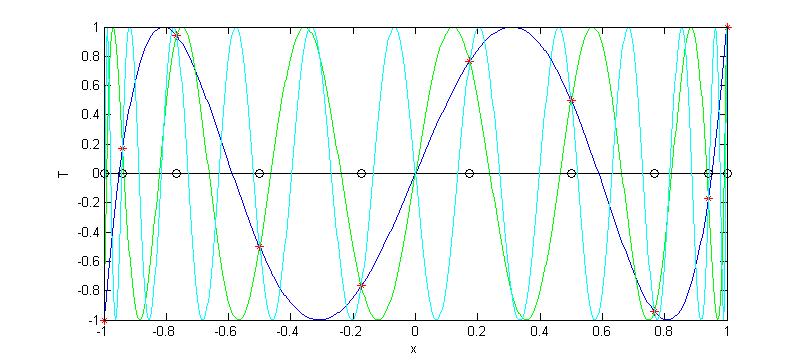
Figure 1: On the CGL grid (open black circles) for N=9 T5 is identical to T13 (green) and T23 (cyan). Points of intersection on the CGL grid are marked with red *'s.
6 Rates of Convergence
Repeatedly integrating equation (5) by parts we
get
|
an = |
1
nm
|
|
2
p
|
|
�
�
|
1
-1
|
(1-x2)-1/2 f(m)(x) Tn(x) dx. |
| (19) |
Thus, if f(x) is m-times (m � 1) continuously
differentiable in [-1,1] the above integral will exist and we
can conclude that
If we make a careful choice of which definition of the integral to
use, the same result can be shown to be true if f(x) is
(m-1)-times differentiable a.e. (almost everywhere) in [-1,1]
with its (m-1)th derivative of bounded variation in [-1,1].
Since the absolute value of each Tk is bounded above by one on
[-1,1], it follows that the truncation error for the continuous
expansion is bounded by the sum of the absolute value of the
neglected coefficients:
|
|f(x) - SN (x) | � |
�
�
n=N+1
|
|an|. |
| (21) |
A similar bound, with an additional factor of two, holds for the
interpolating partial sum:
|
|f(x) - IN (x) | � 2 |
�
�
n=N+1
|
|an| |
| (22) |
for x � [-1,1]. From (20),
(21), and (22) we conclude
that
|
|f(x) - SN (x) | = O(N-m) |
| (23) |
and
|
|f(x) - IN (x) | = O(N-m). |
| (24) |
If f is infinitely differentiable the convergence is faster than
O(N-m) no matter how large we take m. This is
commonly termed spectral accuracy or exponential
accuracy. If f can be extended to an analytic function in a
suitable region of the complex plane, the pointwise error on
[-1,1] can be shown to be
for some r > 1 [14]. In figure
2 the rather slow decay rate of the error
with increasing N is illustrated for the absolute value function
(35) for which m=1. This can be contrasted with
the rapid spectral convergence of the infinitely smooth function
(33) which is also illustrated in figure
2. Notice that the decay of error for the
smooth function ceases at about N=140. This is due to the
accuracy of the representation of floating point numbers on the
computer which limits accuracy to about 14 or 15 decimal places.
No matter what rate of decay the coefficients have, the
convergence rate is only observed for n > n0. Using an
approximation with fewer than n0 terms may result in a very bad
approximation. For example, the decay rate of the coefficients of
the infinitely smooth function in the applet is not yet evident
for N=17 and the approximation is very poor.
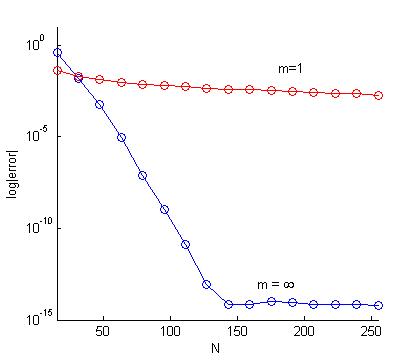
Figure 2: Convergence of an infinitely differentiable function f2(x) = ecos(8x3+1) vs. convergence of a continuous function f5(x)=|x|.
Applet Activity.
Equation (19) allows us to conclude that if
f is a polynomial of degree N, then an = 0 for all
n > N since f(n)(x)=0 n > N. In the CP applet select the
"7th degree polynomial" from the Functions menu. Use the slider
at the bottom of the applet to set N to 9. From the Options
menus check plot coefficients and semiLogY. Observe that ak = 0
(to within machine precision) for n > 7.
If m=0, i.e, f is discontinuous, the accuracy of the Chebyshev
approximation methods reduces to O(1) near the
discontinuity. Sufficiently far away from the discontinuity, the
convergence will be slowed to O(N-1). Oscillations
will be present near the discontinuity and they will not diminish
as N � �. Additionally, the oscillations will not
even be localized near a discontinuity. This situation is referred
to as the Gibbs phenomenon. A nice history of the Gibbs
phenomenon can be found in [12].
Applet Activity.
From the Functions menu select the sign function. From the
Options menus uncheck plot coefficients and check semiLogY. Use
the slider at the bottom of the applet to slowly change N from
10 to 256. Observe that the maximum amplitude of the
overshoot at the discontinuity does not decrease with increasing
N. Observe that sufficiently far away from the discontinuity
that the oscillations are slowly decaying. Now check plot
coefficients on the Options menu and again use the slider at the
bottom of the applet to slowly change N from 10 to 256.
Notice that the coefficients are decaying, but at a very slow
rate. Spectral convergence has been lost due to the
discontinuity. Select the "smooth" function from the Functions
menu and compare how fast the coefficients of this function decay
compared to the sign function.
7 Filters
Spectral filters can be used to enhance the decay rate of the
Chebyshev coefficients [20] and to lessen the effects
of the Gibbs phenomenon. The filtered Chebyshev approximation is
|
FN ( x) = |
N
�
n=0
|
s |
�
�
|
n
N
|
�
�
|
an Tn(x) |
| (26) |
where s is a spectral filter. A pth (p > 1) order
spectral filter is defined as a sufficiently smooth function
satisfying
The convergence rate of the filtered approximation is determined
solely by the order of the filter and the regularity of the
function away from the point of discontinuity.
If p is chosen increasing with N, the filtered expansion
recovers exponential accuracy away from a discontinuity. Assuming
that f(x) has a discontinuity at x0 and setting d(x) = x -x0, the estimate
|
|f(x) - FN(x)| � |
K
d(x)p-1Np-1
|
|
| (30) |
holds where K is a constant. If p is sufficiently large, and
d(x) not too small, the error goes to zero faster than any
finite power of N, i.e. spectral accuracy is recovered. When x
is close to a discontinuity the error increases. If d(x) = O(1/N) then the error estimate is O(1).
Many different filter functions are available, but perhaps the
most versatile and widely used filter is the exponential filter
|
s(w)=exp(-aw2p) p = 1,2,� |
| (31) |
of order 2p. In order for condition (29)
to be satisfied, the parameter a is taken as
a = -lnem where em is defined as
machine zero. On a 32-bit machine using double precision
floating point operations, em=2-52 �
2.2204e-16 and ln(e) � -36.0437.
Applet Activity.
The exponential filter is implemented in the CA applet. The
default order of the filter is 4 (p=2). Select the sign
function from the Functions menu. From the Approximations menu
select the blue interpolation and red filter options. From the
options menu check semiLogY and uncheck connect. Use the slider
to increase N and observe the rapid decrease in the error of the
filtered approximation away from the discontinuity. The filter
has restored spectral accuracy at points sufficiently far away
from the discontinuity. Next, check plot coefficients on the
options menu and compare the filtered and unfiltered coefficients.
Now, display the parameters dialog from the options menu and enter
1 in the filter order box to change the order of the filter to
2. Repeat the above experiments. Observe how the sharp front at
the discontinuity is rounded or smeared in the filtered
approximation by the low order filter. Enter 4 in the filter
order box to change the order of the filter to 8 and repeat.
What do you observe?
Applet Activity.
Select the absolute value function from the Functions menu and
repeat the previous applet activity.
Applet Activity.
The EP applet illustrates the strength of the damping applied in
equation (26) to the coefficients ak from
k=0,1,�,N for filters of order 2 to 32. The slider at the
bottom of the applet can be used to change the order of the
filter. Observe that as the order of the filter increases that
less damping is applied to the coefficients with small k.
8 Applet Example Functions
The example functions included in the applet are the sign
function (m=0)
the "smooth" function (m=�)
the square root function (m=1)
the absolute value function (m=1)
and a seventh degree polynomial
|
f6(x) = x7 - 2x6 + x + 3. |
| (36) |
9 Current Research Area
Chebyshev approximation is an old and rich subject. However, many
areas that employ Chebyshev polynomials have open questions that
have attracted the attention of current researchers. One example
is pseudospectral methods for the numerical solution of partial
differential equations (PDEs). Chebyshev pseudospectral methods,
which are based on the interpolating Chebyshev approximation
(12), are well established as powerful
methods for the numerical solution of PDEs with sufficiently
smooth solutions.
Interpolation means that f(x), the function that is
approximated, is a known function. The terms collocation
and pseudospectral are applied to global polynomial
interpolatory methods for solving differential equations for an
unknown function f(x). Detailed information on pseudospectral
methods may be found in the standard references
[3,6,7,9,10,19].
Many important PDEs have discontinuous (or nearly discontinuous)
solutions. See the article [16] for a discussion of one
such class of PDEs, nonlinear hyperbolic conservation laws. In these
cases, the Chebyshev pseudospectral method produces approximations
that are contaminated with Gibbs oscillations and suffer from the
corresponding loss of spectral accuracy, just like the Chebyshev
interpolation methods that the pseudospectral methods are based on.
An active research area is the development of postprocessing methods
to remove the Gibbs oscillations from PDE solutions and to restore
spectral accuracy. Spectral filters may be used but they perform
poorly in the neighborhood of discontinuities. More sophisticated
methods that do better in the area of discontinuities, but they may
need to know the exact location of the discontinuities. The methods
include Spectral Mollification, Gegenbauer Reconstruction
[11], Padé Filtering, and Digital Total
Variation Filtering. Several postprocessing methods with
applications are discussed in [17] with supporting web
material at http://www.scottsarra.org/signal/signal.html. The
ultimate goal is a "black box" postprocessing algorithm, which can
be given an oscillatory PDE solution and return a postprocessed
solution with spectral accuracy restored.
10 Further Explorations
In addition to the exponential filter, other postprocessing methods
for lessening the effects of the Gibbs phenomenon exist. Explore
some of them which include:
- Other spectral filters. See [2].
- Reprojection methods. Reprojection methods work by
projecting the slowly converging Chebyshev approximation onto
a Gibbs complementary basis in which the convergence is
faster. See [8,11,17].
- Padé based reconstruction. Padé methods
reconstruct the Chebyshev polynomial approximation as a
rational approximation [13].
- Digital Total Variation (DTV) filtering. DTV methods
which were developed in image processing have been used to
postprocess Chebyshev approximations. See [18].
11 Summary
Chebyshev approximation and its relation to polynomial interpolation
at equidistant nodes has been discussed. We have illustrated how the
Chebyshev methods approximate with spectral accuracy for
sufficiently smooth functions and how less smoothness slows down
convergence. We have illustrated how the presence of a
discontinuity leads to lack of convergence at the discontinuity and
leads to slowed convergence away from the discontinuity. We have
described the Gibbs phenomenon which is characterized by a lack of
or slow convergence as well as non-physical oscillations. Spectral
filtering was discussed as a method used to lessen the effects of
the Gibbs phenomenon and to restore spectral accuracy sufficiently
far away from a discontinuity. Postprocessing methods to lessen the
effects of the Gibbs oscillations are an active research area which
would be an excellent topic for undergraduate research or as the
topic of a Masters thesis.
References
- [1]
-
J. Berrut and L. N. Trefethen.
Barycentric lagrange interpolation.
SIAM Review, 46(3):501-517, 2004.
- [2]
-
John P. Boyd.
The Erfc-Log filter and the asymptotics of the Vandeven and
Euler sequence accelerations.
Houston Journal of Mathematics, pages 267-275, 1996.
- [3]
-
John P. Boyd.
Chebyshev and Fourier Spectral Methods.
Dover Publications, Inc, New York, second edition, 2000.
- [4]
-
W. Briggs and V. Henson.
The DFT: An Owner's Manual for the Discrete Fourier
Transform.
SIAM, 1995.
- [5]
-
R. Burden and J. Faires.
Numerical Analysis.
Brooks Cole, eigth edition, 2005.
- [6]
-
Claudio Canuto, M. Y. Hussaini, Alfio Quarteroni, and Thomas A. Zang.
Spectral Methods for Fluid Dynamics.
Springer-Verlag, New York, 1988.
- [7]
-
D. Funaro.
Polynomial Approximation of Differential Equations.
Springer-Verlag, New York, 1992.
- [8]
-
A. Gelb and J. Tanner.
Robust reprojection methods for the resolution of the Gibbs
phenomenon.
To appear in Applied and Computational Harmonic Analysis, 2005.
- [9]
-
David Gottlieb, M. Y. Hussaini, and Steven A. Orszag.
Theory and application of spectral methods.
In R. G. Voigt, D. Gottlieb, and M. Y. Hussaini, editors,
Spectral Methods for Partial Differential Equations, pages 1-54. SIAM,
Philadelphia, 1984.
- [10]
-
David Gottlieb and Steven A. Orszag.
Numerical Analysis of Spectral Methods.
SIAM, Philadelphia, PA, 1977.
- [11]
-
David Gottlieb and Chi-Wang Shu.
On the Gibbs phenomenon and its resolution.
SIAM Review, 39(4):644-668, 1997.
- [12]
-
E. Hewitt and R.E. Hewitt.
The Gibbs-Wilbraham phenomenon: an episode in Fourier analysis.
History of Exact Science, 21:129-160, 1979.
- [13]
-
R. Mace.
Reduction of the Gibbs Phenomenon in Chebyshev approximations
via Chebyshev-Padé filtering.
Master's thesis, Marshall Universigy, 2005.
- [14]
-
J. Mason and D. Handscomb.
Chebyshev Polynomials.
CRC, 2003.
- [15]
-
T. Rivlin.
The Chebyshev Polynomials.
Wiley, 1974.
- [16]
-
S. A. Sarra.
The method of characteristics with applications to conservation laws.
Journal of Online Mathematics and its Applications, 3, 2003.
http://www.joma.org/mathDL/4/?pa=content&sa=viewDocument&nodeId=389
(accessed December 16, 2005).
- [17]
-
S. A. Sarra.
The spectral signal processing suite.
ACM Transactions on Mathematical Software, 29(2):1-23, 2003.
- [18]
-
S. A. Sarra.
Digital total variation filtering as postprocessing for Chebyshev
pseudospectral methods for conservation laws.
To Appear in Numerical Algorithms, 2006.
- [19]
-
L. N. Trefethen.
Spectral Methods in Matlab.
SIAM, Philadelphia, 2000.
- [20]
-
H. Vandeven.
Family of spectral filters for discontinuous problems.
SIAM Journal of Scientific Computing, 6:159-192, 1991.
File translated from
TEX
by
TTH,
version 3.66.
On 16 Dec 2005, 13:33.